Fashion Retail Analytics using PowerBI

The analytics module developed for the fashion industry incorporates the following needs for the end clients:

·         Consolidation of data from various sources such as spreadsheets and other relational databases.

·         Need of the end client to have a consolidated overview from various retail channels such as Retail sales, consignee sales, showroom sales.

·         Flexibility for analysis of the fashion data across various parameters: client, description of the module, style, size and color. The end clients are also looking at analysis across various date/time granularities such as year, year quarter and year month.

The module developed for the fashion industry enables the end clients to do the analysis across any levels of hierarchy. It enables the following:

·         Develop custom KPIs at any level of snapshot(date/time and garment granularity)

·         Enable data consolidation across multiple data sources

·         Flexibility in doing analysis across various views

The value proposition for the product comes as follows:

The benefit matrix of the product for the end client is as follows:

·  The product is looking at ease of deployment, ease of delivery, ease of maintenance.

The grid matrix for percentage calculation is as follows:

·    

                                                                                                                 

·        Based on the 2(two) measures quantity and value the end client should get at least 30 KPIs for percentages across various levels of date/time and product hierarchies.

      Attached are the first set of views for the end client:

    Consolidated dashboard: this view entails the comprehensive overview of metrics and KPIs after the consolidation has been completed. The following are the key tenets for the consolidated dashboard:

·          The view is independent of time

·         The  view is independent of date

Client view for value by year:

In the above view, we are looking at 2(two) separate measures quantity and sales.

In the attached dashboard,

The above is client analysis by fiscal years.

The  above module is the percentage client break up for a given fiscal year.

Thus the team has taken care of percentage snapshots at various levels of hierarchies.

  

Client View for Total Value By Year:

Client View for Total Quantity By Year:

Client View For Value By Quarter:

Client View For Total Quantity By Quarter:

Please contact the following for demo:
Apoorv Chaturvedi: support@mndatasolutions.com;support@turbodaatatool.com
Phone:+91-8802466356

Website; https://mn-business-intelligence-india.business.site/

Turbo Analytics-Batch wise, Bill wise Reports

Turbo Tally Reports

The given product is for the following set of end clients:
a.) Companies looking to give out loans to other firms
b.) Companies looking to factor invoices for other firms
c.) Companies looking for financial advisory services

Background:
The given product has been developed in collaboration with top end financial consultants from Deloitte, Schlumberger. The given product has been developed to provide ease of reporting using Powerbi from desktop solutions such as Tally.

The details of the solution:
o All the reports shall be embedded in Tally
o All the reports have been designed in such a manner that direct integration with databases using
json, xml can be done with ease.
o All the reports can be exported to MS Excel
o Direct integration with PowerBI and Tableau shall be done for ease of analysis.
o The preliminary solution contains 5(five) different reports entailing master details, transaction
details and the payment/receivable ageing details.

For the same the ETL team has devised a solution that entails the following:
 Get complete details of sundry debtors and sundry creditors.
Difference from Tally report:
o The given output shall be a consolidated list of sundry debtors and sundry creditors. The
output can be directly interfaced with any database (cloud or on site relational database).
 Get the complete list of sales, purchase, stock journal, credit notes and debit note outputs. In the
first version the journal details (used for fixed asset purchase) have been excluded.
o Difference from Tally:
 The end client does not need to use multiple reports of sales register, purchase
register and journal register

 Calculate the bill receivable and bill payable ageing details. This is required because the end client
should know the following:
o Outstanding bill payments
o Outstanding bill receipts.

Bill receivable and bill payable ageing report: this particular report captures the following movement
types:
o Sales
o Purchase
o Stock journal debit
o Stock journal credit
o Journal debit
o Journal credit
o Payment
o Receipt
For the given report, the bill reference number is required. The entries that do not have the bill
reference number shall be excluded from the report.
The formulae for the Bill payable ageing as per the product is as follows:
o Total payable outstanding ageing: Total purchase + Total journal debit + Total stock journal debit-
payment - Total debit notes
o Total receivable outstanding specification: Total sales + Total journal credit + Total stock journal
credit - receipt - Total credit notes
Level of granularity of the report: this report has been generated at voucher, allledgerentries and bill
allocations level from the Tally solution. The ageing aggregate has been generated for the consolidated
time period for which Tally has been opened by the end user.

Ageing formulae: the ageing formulae has been devised as the difference between the current fiscal
date as set by the system variable ##SVCurrentdate and the bill due date. The bill due date is the bill
date in case the bill credit period for the sundry debtor or sundry creditor is 0, else it adjusts the bill due
date as per the bill credit period.

In case of On Account entry the following shall be the entries:

·         Due date of payment shall be the same as Bill credit period

·         The number of due days shall be 43830.

·         ‘Name’ in the audit report refers to the bill reference number.

The final report looks as follows:

Attached is the explanation of the above report:

·         DATE: For the sales, purchase invoice

·         BILLID: this is the reference number between sales and receipt, purchase and payment.

·         PARTYLEDGERNAME: self-explanatory

·         TOTAL  OUTSTANDING RECEIVABLES: to date total receivables, that is total sales minus total receipt

·         TOTAL  OUTSTANDING PAYABLES: to date total payables, that is total purchase minus total payments

·         Ageing: this is the number of days between current date and the date of sales/purchase.

Note:

·         This report includes logic for credit notes, debit notes, stock journal and journal also.

The given report has consolidated the following Tally reports:

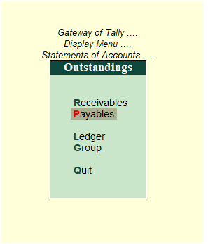
Also the given report helps give the total ledger outstandings across all ledgers. Within Tally the end client is supposed to extract total outstandings ledger wise

Sundry creditors and Sundry debtors reports:

o   The report shall include all sundry creditors and sundry debtors by looking at whether the ledger entries belong to group sundry debtors or group sundry creditors.

o   The report shall include all outputs as in ledger details for sundry debtors and sundry creditors.

Explanation of each field is as follows:

·         PARTY NAME: the party to which sales, purchase, credit note or debit note has been issued

·         ENTITY TYPE:  Select Regular from Registration Types.

·         PAN: Self-explanatory from above screenshot.

·         ADDRESS: Self-explanatory from above screenshot.

·         PINCODE: Self-explanatory from above screenshot.

·         STATE: Self-explanatory from above screenshot.

·         COUNTRY: Self-explanatory from above screenshot.

·         All the other details are coming from ledger master.

Sample Movement analysis report:

This report is built at Voucher and All Ledger Entries details.

In this report, the following is the business logic that is given.

o   The total amount is the first collection field of amount by all ledger entries

o   The taxable amount is the second collection field by all ledger entries

o   For the IGST amount the software checks for the IGST entry in 3^rd, 4^th and 5^th ledgers from voucher details.

o   For the SGST amount the software checks for the 3^rd, 4^th and 5^th ledgers from the voucher details

o   For the CGST amount, the software checks for the 3rd, 4^th and 5^th ledgers from the voucher details.

This given report consolidates 5 different Tally reports as follows:

Explanation of each field is as follows:

·         Partyledgername: the party to which sales, purchase, credit note or debit note has been issued

·         GST registration type: this is the registration type for the second ledger in the voucher as per inventory view.

·         Invoice number

·         Invoice date

·         Ship to: if the voucher has ship to details then the same shall be given

·         Bill to: if the voucher has ‘bill to’ details then the same shall be given

·         PARTYGSTIN: the GST number for the party

·         Document number: the reference document number of the voucher. It could be sales, purchase etc. this is the parent of the voucher type name

·         Currency

·         Note no: to be extensively used for the credit notes and debit notes

·         Total: The total invoice amount

·         Taxable: the total taxable amount

·         IGST, SGST, CGST and CESS: self-explanatory

·         GST supply: specifies whether goods or services

·         Ledger: the second ledger entry in the voucher

·         BasicPurchaseorderno: specifies the basic purchase order based on which the sales invoice was generated

·         GST nature: specifies whether ‘taxable’, ‘exempt’ etc.

·         Basicshipvesselno

·         Basicorderref

·         Basicshippingdate

·         Dispatch date

·         Good receipt date

                                                      

Points to note:

o   The given module does not have HSN details

o   The fields GST Nature of Return, Taxability and nature of services have been set as from the ledger object and associated collections. For the same the collections GST details, State wise details and Rate details have been extensively used.

Quick points to note:

o   If the value are empty then a default value of “NA” has been put into it.

Batch Allocation report: This particular report gives the batch wise profitability across all movement types: sales, purchase, journal debit, journal credit, debit notes and credit notes

This report helps consolidate the different movement type reports from sales, purchase into one single report.

For example instead of a filtered report as given below:

The end client shall get a consolidate batch movement report.

The explanation for the report is as follows:

·         Batch ID: Self explanatory

·         Batch name: Self explanatory

·         Billedqty_purchase: Total quantity purchased for the given batch to date

·         Billedqty_sale: Total quantity sale for the given batch and given item to date

·         Batchqty_stock: Total stock journal debit for the batch and given item up to the given date

·         Batchqty_stock_Jrnl: Total stock journal credit for the batch  and item up to the given date

·         Debit_Note: Total debit note quantity for the item and batch up to the given date

·         Credit_Note: Total credit note quantity for the item and batch up to the given date

·         Net_Difference:Billedqty_purchase-Billedqty_sale+Batchqty_stock-Batchqty_stock_jrnl-debit_Note+Credit_Note

·         Batch_Rate: This is the purchase rate of the item for the given batch

·         Net_Amount: Multiplication of Batch_rate with Net_Difference

     Prepared by:

     Contact: Apoorv Chaturvedi(8802466356)

    email:mndatasolutionsindia@gmail.com,support@mndatasolutions.com;support@turbodatatool.com

  Website: https://mn-business-intelligence-india.business.site/

                                                                                        

MARKET BASKET ANALYSIS-TURBODATA

 

Market Basket  Analysis is a modelling  technique based upon the  theory that if we buy  “ ITEM A” then there is a probability of buying “ITEM B”.

Purpose of Market Basket Analysis  through Turbodata

The purpose of market basket analysis is to determine what products customer purchase together .i.e. if a customer purchases milk  then there is possibility that the customer will also buy  sugar.MBA(Market basket analysis) is used to analyze the customer behavior.

Why Market Basket Analysis in Turbodata?

·       Data has been cleansed and consolidated in Turbodata.

·       Maximum data redundancies have been removed and joins have been minimized. All the business logic from the ERPs has been pre coded. This process helps us in the following ways:

o   The reporting team can use parameterized queries to get the required outputs. There is no need to store all the data in pre aggregated form. This is important since there are a large number of item combinations that are possible

o   Turbodata’s market basket analysis solution offers analysis at the reporting layer without the use of expensive reporting tools.

o   The solution is available in both Tableau and PowerBI.

o   Multiple users can access  the report. Turbodata offers analysis at any point in time, across any number of locations or any combination of items.

o   Facility for large scale deployment of the code because of the usage of table variables and functions.

STEPS:

STEP1  : A  master procedure with two input parameters was created with date.

STEP 2:  Five variables was created for the  calculation of confidence ,lift and support.

·       @n_total :total  number of order

·       @n_dual: number of invoices having more than ONE item

·       @n_item1:number of invoices having ITEM1

·       @n_item2: number of invoices having ITEM2

·       @n_item1_item2: number of invoices having both ITEM1 and ITEM2.

STEP 3: Calculate Confidence , Support and Lift value.

So for this we have been created a function instead of procedure because:

·       Function is compiled and executed every time whenever it is called .It is just like a formula we use.

·       We can add the parameter according to the requirement.

·       When we need only input parameter.

There are two types of function we use  in our code

1.    Scalar valued  function

2.    Table valued function

   Scalar valued function

Scalar valued function are used when we have to returns  a single value(integer,decimal or any).it might or might not be related to tables in our database.

   Table valued function

Table valued function returns the specified columns for row in our table meeting the given criteria.

So for the above process  we use the following solutions:

   Calculation of @n_total

N_total is the sum of total orders.Total number of orders should be come from  item_supplier_order at a particular date.so we join item_supplier_order table with dim_date and we take only that date which is less than or equal to the @date.

Here is the snapshot for total order.

   Calculation  for@n_dual

 This is the function which we have been created for invoices having more than one order.Here we need partyledgername from item_supplier_order,item  from item_sales_order and date from dim_date.so we join item_supplier_order  with item_sales_order on the basis of composite key ,the result will further join with dim date.

For more than one item we take the count of dim_item_id having count greater than one.

Attached is the snapshot from the Turbodata:

   Calculation for @n_item1

This is the function we created for the item1.

We took order_no from item_supplier_order,dim_item_id from item_sales_order  and item from dim_item having the condition that count of dim_item_id is greater than one.

   Calculation for @n_item2

The similar process is used for the calculation for item2 as we have been done for item1

      Calculation for both the items @n_item1_item2

                      This is the function created for both the ITEM1 and ITEM2.

   Confidence is defined as division of the frequency of both the item to item1.

i.e., Confidence=@n_item1_item2/@n_item1

   Support  is defined as the division of occurrence of both the items to total.

i.e  support=2n_item1_item2/@n_total

   Lift is defined as the division of the support of both the item to muliplication of support A and support B.

i.e  Lift =@support/@support_x * @support_y

How the Market Basket Analysis code has been developed over compressed database.

How Turbodata helped lower the costs of developing a datawarehouse and helped the end clients do predictive analytics with quickness and ease-applicable for retail sales and inventory(Website: www.mnnbi.com)

Purpose of the development of the product: The Turbodata team intends to reduce the costs of the analytic solutions by creating a single platform for ETL, Reporting, Reporting development and predictive analytics. The team also intends to provide the best in class analytics on the same machine on which the ERP is running or with the addition of minimum hardware requirements for the end client. This has been done to develop scalable systems that can be deployed over a large number of customers(with limited budgets) with ease(deployment, delivery and usage) and convenience(maintenance).

The end goal is to increase derisking and predictability for the end clients at lower costs.

Methodology for achieving the required ends for the end client:

·         Turbodata adopted the Inmon methodology for datawarehouse development so that multiple data sources could be added onto the same datawarehouse. That is the change from one data source to another was done with ease. More details on the attached web page link: http://mnnbi.com/mnnbi_tallydataconsolidation.html

o   The benefits of the normalization of data were as follows:

§  The incremental data load took minimum time and had minimum impact on the source system. The ETL team was able to commit the incremental data load to a maximum of 2GB RAM from multiple source systems. The source systems did not hang with the incremental data load working.

§  Error handling was done with ease at staging layer.

§  Massive data compression took place due to reduced data redundancies.

§  The business logic was coded between staging and the ODS layers thereby reducing the length of the final sql code.

The attached video shows a more detailed description of the benefits listed above:

https://www.youtube.com/watch?v=k9Oe9EDRfTM&feature=youtu.be

The joins were reduced in the data mart layer(over which a reporting layer was built).

The ETL team was able to develop extremely complex reports using the datawarehouse as in the attached sample:

https://www.youtube.com/watch?v=1ySNrgI4Na0&feature=youtu.be

Due to the data compression for most projects the ETL team are able to bring the data within 1 GB. Hence the desktop version of Microsoft Power BI could be used free of cost for the end client.

Reducing the cost of predictive analytics solutions

 Most of the end clients use high end predictive tools over the datawarehouse/ over the direct data extract from various source databases. With large datasets predictive analytics using in memory solutions entails high usage of RAM. The ETL team has gone around this issue in the following manner:

o   A seamless environment was created for ETL, reporting and thereafter predictive analytics on SQL/C# and .Net. The reasons for the same are attached herewith:

§  Maintenance becomes easier since there is a single platform for all aspects.

§  The cost comes down since the resources to be used for ETL can also be used for predictive analytics

§  Error handling becomes very easy since errors can be captured before in the

Hypothesis testing

Based on the hypothesis testing, the ETL team developed ARIMA analysis and Market Basket analysis in SQL using seamless integrated set of stored procedures. That is the ARIMA analysis flowed from the datawarehouse A,B,C categorization. The ETL team thus reduced the requirement for high end R and Python developers to code over the datawarehouse thereby presenting a seamless solution to the end client on a 8GB RAM machine.

Benefits to the end client:

·         The end client gets immediate and confirmed peace of mind and satisfaction through immediate deployment of predictive and forecasting analytics modules.

·         No additional hardware/software requirements need to be taken

·         The costs are way lower for the end client.

·         Large scale deployment is possible with the given set of solutions.

Please check the attached video for the same:

https://www.youtube.com/watch?v=PQfsfWLkaP8&feature=youtu.be

A more detailed video is attached herewith:

https://www.youtube.com/watch?v=7DoZDBay-bQ

Example of predictive analytics with Turbodata: Example of predictive analytics-Turbodata

Market Basket Analysis through PowerBI

The PowerBI code has been developed to enable the following:·       Run the market basket analysis code based on 2 input item parameters across any filter date and location ranges.
·       Removes the dependence on SQL server for the implementation of Market basket analysis.
·       Faster execution times since the measures and columns are calculated on a columnar basis instead of row by row basis.
The attached is the methodology of Market basket analysis using PowerBI over Turbodata

Step 1:Import the  file from SQL server.

Step2:Three parameters are declared.i.e. item_1,item_2,date_1.This has been done through Power Query Editor.

For creating parameters:

·       Open power query editor

·       Go to manage parameter

·       Create a parameter

Set the parameter of date_1 in item_supplier_order

Step 3:we have to calculate support,confidence and lift value.

calculation of support :

Support=f(X,Y)/total

Where f(X,Y) is the instances of occurrance both the “ITEM A” and ”ITEM B” in the invoices for the given time period.

Total is the count of the total sales order nos. for the given time period

Attached is the snapshot from dax function for f(X,Y):

Snapshot for total:

Snapshot for the calculation of support:

 Snapshot for the calculation of item A only:

Calculation for the confidence:

 Confidence =F(X,Y)/F(X)

Snapshot for the calculation of confidence:

Where P_X_Y is the occurrence of both the item

And P_X is the order no where there is item A.

Snapshot for the calculation of P_X:

Calculation for lift:

Lift =support_1/(support_x*support_y)

Where  support_x  =f(X)/total

Support_y=f(Y)/total

Snapshot for the calculation of lift value:

Snapshot for the calculation of support_x:

Snapshot for the calculation of support_y:

Attached is the summary of final output for the given set of input items(CPU and ALMIRAH).

Market Basket Analysis through Tableau

Market Basket Analysis has been done through Tableau .

There are four data sources we have been taken for the calculation of market basket analysis.

1.    CPU

2.    ALMIRAH

3.    MARKET_BASKET

4.    ORDER_MASTER

We have to calculate the lift,confidence and support value in Market Basket Analysis.So we  have  take the two items ‘CPU’ and ‘ALMIRAH’.

Make three parameters.

1.    Date_1

2.    Item_1

3.    Item_2

We have take the order no. where the CPU has been purchased.

So we join the item_supplier_order with item_sales order on the basis of item_supplier_order_id , dim_date with dim_date_id and dim_item with dim_item_id.

We have pass the parameter through Custom SQL.

Attached is the snapshot from the Tableau for the date parameter:

Similarly attached is the snapshot from Custom SQL to pass the item_1(CPU) parameter:

Attached is the snapshot from Custom SQL to pass the item_2(ALMIRAH) parameter:

This is the another database for the calculation of order_No where almirah are purchased.

MARKET_BASKET is the database where we calculate the order no where both item_1 and item_2 both are purchased.i.e. “ALMIRAH”,”CPU”.

This database is used to calculate total number of invoices(order_no).

For the calculation of the order_no of item_1 we have taken the count distinct of item_1

For the calculation of the order_no of item_2 we have taken the count distinct of item_2

Attached is the snapshot for the calculation of the order_no for both the  item_1 and item_2.

Attached is the calculation for the total order_no.

Based on the above calculation we calculate the confidence ,lift and support value.

Attached is the snapshot for the  calculation of confidence:

Confidence is the value that if a customer purchase item “A” then what likelihood  he will buy item “B”.

Attached is the snapshot for the  calculation of support:

Support value calculation for how the strong is the base.

Attached is the snapshot for the  calculation of lift:

Attached is the snapshot of the resultant:

We take two items “CPU” and ”ALMIRAH” which cannot be a combo so its lift value is less than 1.

Note:

Lower the value of lift lower is the strength of the combo and higher the value of lift higher is the strength of the combo that customer like.

ARIMA model in R

Data is made of noise and signal .

In short time period the probability of noise in the data is greater than signal. For e.g. if we analyze the data on hourly basis ,the  probability of noise is 99.5% and that of signal is 0.5%.

In long time period , the proportion of noise reduces and the proportion of signal increases.For e.g. if we analyze the data on monthly basis, probability of noise could be 50% and that of signal is 50%.

The purpose of tike series forecasting is to segregate the noise from the signal for better management decision making.

ARIMA  stands for :

AR:Auto regressive(p)

Y(t)= c+alpha*y(t-1): Understand the time dependency

I:integration(d)

Y(t)= c+alpha*y(t-1)+beta*y(t-2)+error: understand behavior of error term. Check for stationarity(check whether error is hiding signal patterns).

MA :Moving Average(q)

Y(T)=c+alpha*e(t)+beta*e(t-1). MA indicates the dependence of y(t) on the errors in the previous time periods

Components of ARIMA Model:

}  Trend: A long-term increase or decrease in the data is referred to as a trend. It is not necessarily linear. It is the underlying pattern in the data over time.

}  Seasonal: When a series is influenced by seasonal factors i.e. quarter of the year, month or days of a week seasonality exists in the series. It is always of a fixed and known period. E.g. – A sudden rise in sales during Christmas, etc.

}  Cyclicity: When data exhibit rises and falls that are not of the fixed period we call it a cyclic pattern. For e.g. – duration of these fluctuations is usually of at least 2 years.

Assumption of ARIMA model

·        Data should be stationary: the error terms should not have time dependency

·        Data should be univariate: the regression model is based on only one variable.

Sample code:

data = read.csv('http://ucanalytics.com/blogs/wp-content/uploads/2015/06/sample_data.csv')

data = ts(data[,2],start = c(2003,1),frequency = 12)

plot(data, xlab='Years', ylab = 'sample)

The above code is from R. it reads the data which is csv type. ’ts’ is the time series function which reads the data starting from  first month of 2003 and read plot the data of every month.

Where x-axis is for the “years” and y-axis is for the “sample”.

plot(diff(data),ylab='Differenced sample Sales')

This is  for the difference of y(t)-y(t-1).

plot(log10(data),ylab='Log (sample Sales)')

This graph is for the log value of given sample sale.

plot(diff(log10(data)),ylab='Differenced Log (sample Sales)')              

This graph is for the log difference of sample sales.

ACF:ACF stands for auto-correlation function. It describes how well the present value of the series is related with its past values. A time series can have components like trend, seasonality, cyclic and residual. ACF considers all these components while finding correlations hence it’s a ‘complete auto-correlation plot’.

PACF:PACF stands  for partial auto correlation function. Basically instead of finding correlations of present with lags like ACF, it finds correlation of the residuals. So if there is any hidden information in the residual which can be modeled by the next lag, we might get a good correlation and we will keep that next lag as a feature while modeling.

Attached is the code :

par(mfrow = c(1,2))

acf(ts(diff(log10(data))),main='ACF sample Sales')

pacf(ts(diff(log10(data))),main='PACF sample Sales')

Epilogue

The ETL team has been inspired by the following management books:

·         ‘Profit Beyond Measure’ by Thomas Johnson and Anders Brohms

·         McKinsey Mind by Ethan Rasiel and Paul Friga.

·         Blue Ocean Strategy by W. Chan Kim and Renee Mauborgne

·         Better India, Better World by Narayana Murthy

In case of any requirements please contact the following:

Name: Apoorv Chaturvedi

Email: support@mndatasolutions.com;mndatasolutionsindia@gmail.com;support@turbodatatool.com

Phone: +91-8802466356